Some Definitions
Epochs and Periods
As much as possible, and without becoming too abstract, Cassandra strives to be domain agnostic. That means you should be able to use Cassandra for any type of infrastructure network or component. Whether you are modelling a road network, a group of recreational facilities, a bridge network, a water-pipe network or a rail network: Cassandra should be easy to use without being tied to terminology used mainly for one type of infrastructure.
To this end, we have avoided expressing modelling periods as ‘years’, since for some types of infrastructure a modelling period may be a month or a quarter of a year.
Cassandra has adopted the terminology of ‘epochs’ and ‘periods’ as often used in the context of Markov Chains and Markov Decision Processes (Sheskin 2011). The figure below explains the concepts of epochs and periods:
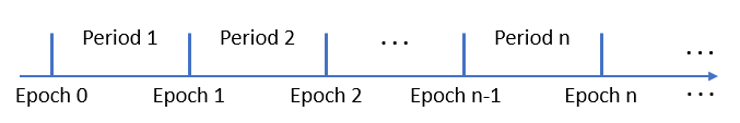
In the context of IDM, and as implemented in Cassandra, an epoch marks the end of a time period. Changes (such as deterioration of elements) happen during a period. Similarly, interventions/treatments are applied during a period.
An epoch marks the END of a period. Thus, Epoch 1 marks the end of Period 1. When Cassandra gives a report showing the breakdown of condition, it will be in terms of epochs. A breakdown of network/facility condition shown for epoch X will therefore reflect the condition at the end of period X.
After the model Initialisation step is completed (see Figure 1 above), the information for each parameter is set for Epoch 0. Model incrementing now starts and after Period 1 the updated information for each parameter is held for Epoch 2, and so forth.
By contrast to a condition status, spending takes place during a period and therefore spending will be reported against periods, not epochs.
The above figure and definitions mean that, when it comes to forecasts of condition, there will always be one more epoch than there are periods. This is because the model has to start off with an initial state in epoch 0, but it has no knowledge of what happened in period 0 because a Cassandra model only applies treatments and makes decisions from period 1 onwards.
When you configure a Cassandra model, you will set the number of modelling periods over which you want the model to run. You do this in the General Settings for the model (see @ref(#gen-settings) for details).
Broad Model Types
In the sections below, we explain what we mean with different model types in the Cassandra context. Please note that each of the model types may have variations depending on certain options and customisations.
Forecast Model
In the Cassandra context, a forecast model is a model that does not do any triggering of treatments, but only does a prediction of future condition with or without a set of associated treatments. Y
ou can use a forecast model to predict the likely future condition of an asset or a network of assets given a specified set of treatments in different periods [^1]. If the set of treatments is empty, we call this a Do-Nothing forecast.
Treatment Selection Model
In the Cassandra context, a Treatment Selection model is a model that uses a custom trigger function to trigger one or more candidate treatment strategies for elements in your model set. The model will then perform heuristic optimisation using either Cost-Benefit Analysis (BCA) or Multi-Criteria Decision Analysis (MCDA) methods.
Decision Making Approaches
The International Infrastructure Management Manual (IIMM) (IPWEA 2020) identifies four main approaches to decision making in the infrastructure management context:
- Net Present Value (NPV) analysis;
- Benefit Cost Analysis (BCA);
- Cost Effectiveness Analysis (CEA); and
- Multi-Criteria Decision Analysis (MCDA).
The IIMM discusses the advantages and disadvantages of these four approaches in great depth. The IIMM suggests that BCA is an extension of NPV (IPWEA 2020). However, in our view NPV is simply one approach within BCA (some others being the maximizing of benefit-cost ratios and incremental cost-benefit ratio methods).
As suggested in the IIMM (IPWEA 2020), the first three approaches require that non-financial outcomes be readily quantifiable. In our experience the quantification of benefits in monetary terms is not only complex, but invariably involves a degree of subjectivity. This subtracts from the value of approaches that rely on a quantification of benefits - whether in direct monetary terms or as a relative indicator of benefits.
Furthermore, in each of the first three approaches, the cost of the treatment alternatives plays a significant, perhaps even dominating, role. It is difficult within the first three approaches to temper the role that cost plays in decision making that involves multiple objectives, as is the case with most network level analyses of infrastructure assets. In MCDA approaches, cost can be made to be simply one of many considerations. Thus, in MCDA it is easier and less complex to increase or decrease the relative importance of cost in the decision-making scheme.