Inverse Distribution
Purpose
To model values from a typical distribution for infrastructure components using the Inverse Transform Sampling method.
The idea behind this function is use the above technique, together with a typical, known distrubution of values, to convert a probability value (ranging from zero to 1) to a value from the distribution.
For example, assume you have a logistic regression model that gives you the probability that for a certain distress (let’s assume rut depth on a road) rapid deterioration will be observed. We then make the assumption that the deterioration increment will be related to the probability of rapid deterioration as shown below:
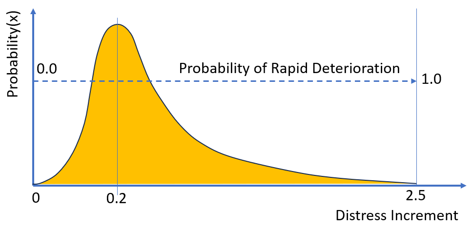
In the above figure we have a typical right-skewed distribution with a maximum around 2.5 and a central tendency around 0.2. We show the (assumed) relation between probability of observing rapid distress development, and the distress increment. Here, ‘probability of observing rapid distress’ could be defined in many ways depending on the domain. For example, it could mean ‘having more than 8 mm rut in less than 5 years’.
If the probability for rapid distress development is high (close to 1.0), we will translate this to an increment around 2.5. If the probability for rapid distress is low (say around 0.1), we will assume an increment around 0.1 to 0.2. But the important point is that this JFunction will ensure that the increments estimated will follow the assumed distribution shape.
You may ask why do we not simply estimate the increment directly instead of using a probability. The reason is that it is often not possible to develop a calibrated model for distress increments unless you have a large data set. Also, small increments may include a significant degree of random error making it difficult to separate random and non-random effects.
In such cases, it may be much easier to identify situations in which rapid deterioration occurred since these are more clearly present (or not). For example, you could set a threshold that identifies all components that reached a certain level of distress within a given age or years in use. Then you can use that data to develop a logistic regression model that can give you a probability of observing rapid deterioration.
In this approach, you do not need multiple years’ data - a single snapshot can be used to develop such a logistic regression model. The only challenge now is how to convert this probability to a distress increment - which is the purpose of this JFunction.
Type Name
‘inverse_distribution’
Definition Syntax
‘[distribution_code] : [scale_factor] : [value_key]’
where:
- ‘distribution_code’ is a code ‘a’, ‘b’, ‘c’ or ‘d’ indicating the type of distribution you want to use. Each code maps to a different distribution shape (see details below).
- ‘scale_factor’ is a number that defines the central tendency or scaling factor for the distribution.
- ‘value_key’ denotes the key mapping to the probability value in the value dictionary. This key should map to a function or value that is in the range of zero to 1.
Note that currently the value you supply for ‘scale_factor’ must be a number and can not be a key mapping to a value in the value dictionary. This constraint will be removed in future upgrades if requested by users.
Example
‘a : 2.5 : f_naasra_proba’
This will use distribution shape ‘a’ (see below) with a central tendency assumed to be at 2.5. It will then convert the probability value contained in key ‘f_naasra_proba’ to a relative increment from the ‘a’ type distribution.
All four the distribution types range from 0 to 10 before adjustment based on the scaling factor value you specify. To simulate, for example, a rut increment distribution with a central tendency at 0.25 mm per year, specify a ‘scaling_factor’ of 0.25. This will adjust the maximum value to be 10 times the central tendency, thus the maximum value will adjust from 10 to 2.5 mm per year and the central tendency will be 0.25 mm/year (for distribution type ‘a’).
Distribution Types
Distribution Type ‘a’
This distribution is a typical right-skewed distribution ranging from zero to 10 if the central tendency is specified at 1.0. This distribution is, for example, suitable for simulating a rut increment if properly adjusted with a central tendency that suits an observed value. This distribution has zero frequency at probability zero.
For this distribution, the scaling factor determines the central tendency for the distribution.
Distribution Type ‘b’
This distribution is a typical right-skewed distribution ranging from zero to 10 if the central tendency is specified at 1.0. This distribution is, for example, suitable for simulating a rut increment if properly adjusted with a central tendency that suits an observed value. This distribution does NOT have zero frequency at probability zero. Compared to type ‘a’ this distribution is slightly more right-skewed and more approximates an exponential distribution.
For this distribution, the scaling factor determines the central tendency for the distribution.
Distribution Type ‘c’
This distribution is a severely right-skewed distribution ranging from zero to 10 if the central tendency at 1.0 if the central_tendency_value is set to 0.5. This distribution is, for example, suitable for simulating a roughness increment if properly adjusted with a central tendency that suits an observed value. This distribution does NOT have zero frequency at probability zero.
For this distribution, the scaling factor determines the central tendency for the distribution.
Distribution Type ‘e’
This distribution is a near-explonential distribution ranging from zero to 10 if the central tendency at zero. Suitable for simularing roughness increments if properly adjusted using the ‘central_tendency_value’ which in this case is simply a calibration coefficient. This distribution does NOT have zero frequency at probability zero.
For this distribution, the scaling factor determines the distribution range which will range from zero to 10 times the value you provide for the scaling factor.
For example, for this distribution, to simulate a near exponential Naasra roughness increment distribution with a central tendency at zero and ranging from 0 to 25 counts/year, pass the scaling factor = 2.5. This will adjust the maximum value to be 10 times 2.5 thus 25 Naasra counts per year.
This JFunction type is powerful but somewhat specialised and also limited by the four default distribution types available. If you want to explore using this JFunction to mimic increments from the available distributions, we recommend you set up an dummy input set of around 10,000 rows with probability values ranging from zero to 1.0. Then you can use this function to convert the probability values to increments which you store in a model parameter.
Next, run your model for 1 period, then analyse the parameter outputs for Epoch 1 using a histogram. You can play around with distributions ‘a’, ‘b’, ‘c’ and ‘d’ and also with different values for your ‘scaling_factor’ to see the influence these have on your simulated increments.