Overview

Overview of JFunctions

Juno Functions, or ‘JFunctions’ are a compact way to define the logic and mathematical functions to use in your domain models. JFunctions are defined in plain text, with each JFunction stored as a line in a table containing all your JFunctions. All of your JFunctions combined make up a Function Set. At run-time, JCass loads the function set and parses each JFunction to create a flow of calculations that express your model logic.

This sounds a bit abstract, and it is certainly not an easy concept to master. However, to ensure that JFunctions are powerful enough to achieve what most modellers want to achieve, a certain level of abstraction and complexity is unavoidable.

It always helps to remember that JFunctions are exactly what the name says: Juno Functions. That is, a logical or mathematical function that takes certain inputs and gives out a transformed output.

There are many types of JFunctions. Each function was designed to achieve a certain transformation or logic to serve as a building block for your domain models. When you put a lot of these building blocks together and execute them in sequence (with each output serving as inputs to the next function) you can build highly sophisticated domain models.

The main categories of JFunctions are listed below:

• Basic (Constant, Value Copy, Max-Value, Min-Value
• Text Manipulation (Split-and-Select and Concatenate).
• Counts over/under Thresholds.
• Equalities (Basic Equality, AND compounded, OR compounded).
• Conditional Statements (If-Else and Multiple-If)
• Lookup functions
• Equations (additive equation, ).
• Sum-Product.
• Speciality/Engineering (Date-to-Age, Cost354-Index, Piecewise-Linear, S-Progression, etc.)
• Machine Learning Models

Each of the categories of JFunctions noted above will be explained in detail, with examples, in the sections that follow.

How you Define JFunctions

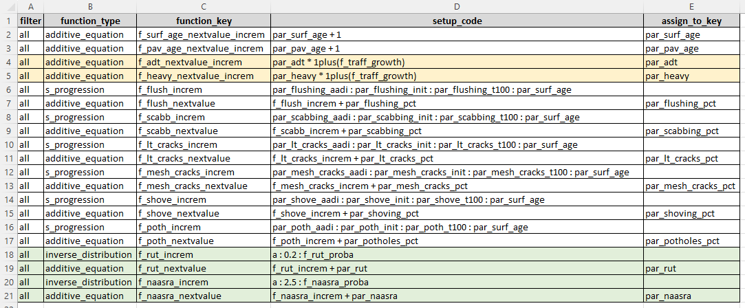
You define your JFunctions in plain text. A logical group of JFunctions (for example, to express a trigger condition) is typically labelled using a distinct Function Block Name. The Function Set that contains the logic for your Domain Model can be edited in an Excel spreadsheet template, as shown below. The template is then imported and saved against your domain model.

Note that the order in which the JFunctions are defined is important. At run-time, the JFunctions will be executed from top to bottom. JFunction keys that are used in a JFunction need to be defined before they are referenced. This concept is explained in more detail in the section below.

The figure below shows a typical set of JFunctions. As shown in the figure, there are columns such as ‘filter’ that you can use to view groups of JFunctions while you edit or build your domain model. You can also colour code groups of rows and this colour coding will be retained when you import or export your Function Set.

Example of a JFunction Definition Set

Data your JFunctions Can Use

Before we delve into the details of how JFunctions work, we need to explain what data is made available to your JFunctions and how you access this data to make your JFunctions work.

In the earlier section dealing with the Framework Modelling Engine we discussed the key steps that the modelling engine executes during a model run. In another section we also discussed the data components associated with a model. If you have not yet studied these two earlier sections - please do so now.

Before proceeding, you should be clear about the four different stages of a model cycle (initialisation, triggering, incrementing and resetting). You should also clearly understand the two main data components involved in a model run (Raw Input data and Model Parameter data).

For those who prefer videos to reading, the video below provides a discussion of the concepts discussed below:

Given an understanding of these concepts, we will now elaborate on the example data shown in Figure 3 in the section dealing with data components.

Example of Raw Input data vs Model Parameter Data

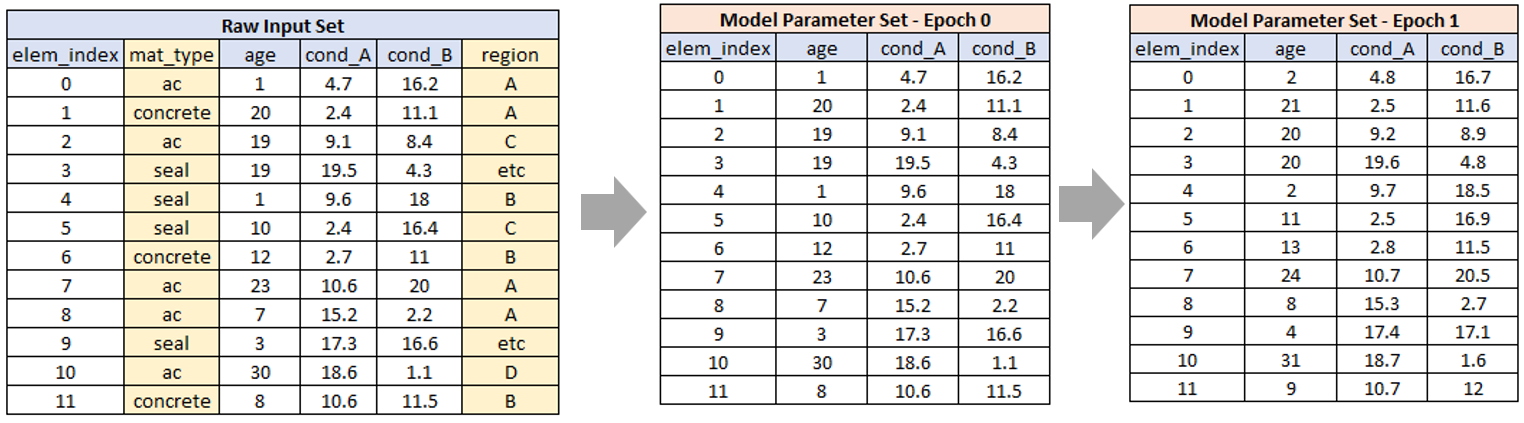
It was explained in the section on the framework model that during a model run, the model loops over all model elements (i.e. the rows in the above figure). In each loop, the model passes to your domain model (the ‘customiser’) both the raw data row and the model parameter row for the current element.

The Value Dictionary

These data are made available to your JFunctions in the form of dictionary of keys and values. You can view this dictionary as a transformed and combined version of the raw data and parameter data for the current element. This is shown conceptually in the figure below for element index 10 from the above figure.

Figure 1. Dictionary of Key-Value Data for JFunctions

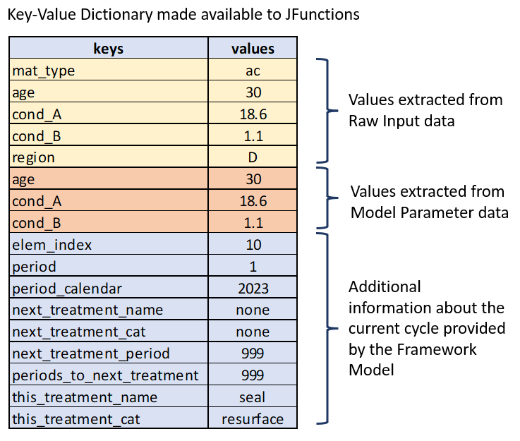
As you can see from the above figure, the dictionary of keys and matching values that is made available to your JFunctions consist of three groups of data: (a) keys and values related to your raw input data; (b) keys and values related to your model parameters; and (c) keys and values containing additional information that is provided by the Framework Model.

While you should understand by now where the raw data and model parameter data come from, the last category of information needs further explanation. While the model runs, it keeps track of certain global variables that are not part of your raw input or model parameter data. As shown in the figure above, this information includes aspects such as the current model period, the name of the next treatment (most likely a committed treatment), or the name of the current treatment (if a treatment was assigned in the current period).

This additional information can thus also be used by your JFunctions to make decisions, calculate increments or resets and so forth. For more information on the Special Key-Value pairs added for you by the model, please see this page

How JFunctions Access Data

Now that you understand how the Framework Model extracts data and and turns it into a dictionary of keys with matching values, we can provide an example of how a JFunction can access this dictionary.

Consider the following JFunction which is a simple equality.

t: mat_type = Concrete : TRUE

This JFunction definition for an equality has several components delimited by a colon (‘:’). Each component of the definition tells JCass, respectively, that:

1. The equality should assume text values (indicated by ‘t:’)
2. The equality is ‘mat_type = Concrete’
3. The comparison is case-sensitive (indicated by the ‘:TRUE’ at the end of the definition code.)

Note specifically that the equality uses the codes ‘mat_type’ and ‘Concrete’. When interpreting this equality statement, JCass will first try to map the codes to one of the keys in the dictionary of values. If a matching key is found, it will use the value matching that key in the evaluation of the function. If a matching key is not found, it will use the code literally.

So, for the example dictionary shown above, we can see that the one of the raw data fields is called ‘mat_type’ and it has a matching value of ‘ac’. There is no key matching ‘concrete’ and therefore the value ‘concrete’ is interpreted literally.

So the above JFunction will be evaluated by JCass as:

ac = Concrete (using a case-sensitive evaluation).

Clearly, this statement is false, and therefore the above JFunction will return a 0 (zero) which means ‘false’.

If our equality JFunction was defined as follows:

t: mat_type = AC : FALSE

then this will evaluate to a 1 (true) because the value matching key ‘mat_type’ is ‘ac’ and we are not making a case-sensitive comparison (as indicated by ‘: FALSE’ at the end of the function definition code).

JFunctions Keys

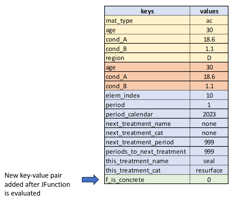
As mentioned in the above section on how you define JFunctions and as shown in the example figure, each JFunction is defined with a ‘function_key’. For example, in the equality example shown above, we may assign the key ‘f_is_concrete’ to the JFunction. When the JFunction is evaluated, it will add a new key-value pair to the function data for the current element, so that the data dictionary that is used by further downstream JFunction elements can make use of this result.

So after the equality with the key ‘f_is_concrete’ has evaluated, the dictionary shown above will now look like this (assuming the result was false/zero):

Figure 2: Updated Dictionary of Key-Value Data

Example: Sequential Calculation

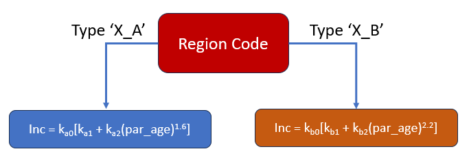
Let us now consider a simple example of a decision workflow which we assume is one of the building blocks of a Domain Model decision workflow. For this example, we assume that there is a code called a ‘Region Code’ which determines how fast an element will deteriorate. We assume there are only two main region codes, namely ‘X_A’ and ‘X_B’.

The decision logic is shown in the figure below. We assume the region code is constructed by concatenating two fields from our raw data file: (a) ‘sub_region’ and (b) ‘climate’. Once we know the region code, we need to calculate the rate of deterioration which is the increment (‘inc’). We assume there are two different increment equations for region codes ‘X_A’ and ‘A_B’ respectively.

Figure 3: Decision Workflow Example

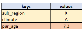
The data that is made available by JCass for the JFunction processes is shown below.

Figure 4: Decision Workflow Example

To execute this logic, we will sequentially construct the building blocks with which to do the calculations. We need the following JFunctions:

1. We use the ‘Concatenate’ function to concatenate the values in fields ‘sub_region’ and ‘climate’ using an underscore to join the values.
2. We define the constants for both equations as ‘Constant’ JFunction types. We need one JFunction for each constant (k_a0, k_a1, k_a2 and k_b0, k_b1, k_b2).
3. We need two ‘Additive Equation’ type JFunctions to define the increments for region codes ‘X_A’ and ‘A_B’.
4. We need an “IfElse” JFunction to determine which of the above two additive equations will determine the final increment.

Assuming the above dictionary of data, our JFunction set for this logic will look as follows:

Figure 5: JFunctions for Workflow Example

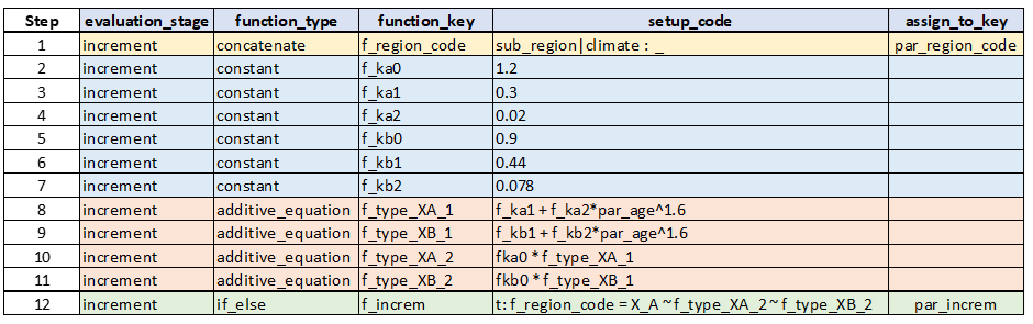
For now, do not concern yourself too much with the syntax of the setup code for the various JFunctions. You can study this later by looking at the detailed documentation for each JFunction. Just focusing on the steps in the JFunction logic, we can see the following steps (shown in the Figure above):

Step 1: We create a region code by concatenating data in the raw data fields ‘sub_region’ and ‘climate’. We assume the data is such that this should give us either ‘X_A’ or ‘X_B’.

Steps 2 to 7: We add all of the constants needed for the two equations.

Steps 8 and 9: We create the inner part of the increment equations for region codes ‘X_A’ and ‘X_B’, respectively.

Steps 10 and 11: We multiply the inner parts calculated in Steps 8 and 9 with the two calibration constants k_a0 and k_b0 for region codes ‘X_A’ and ‘X_B’, respectively.

Step 12: We use an If-Else function to assign the correct result (either ‘f_type_XA_2’ or ‘f_type_XB_2’) depending on whether or not the region code is ‘X_A’.

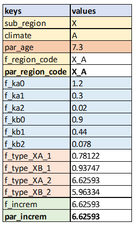
Remember that JFunctions evaluate from top to bottom, so as each JFunction is calculated the dictionary of parameter values will be updated so that downstream JFunctions can access the data. So for example, when the execution is finished up to step 9, the dictionary of parameter values will look like this:

Figure 6: JFunctions for Workflow Example

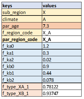
We will leave it to you to confirm the calculated values are correct based on the equations shown in the decision structure shown in the Figure 3 above.

You can see from the ‘assign_to_key’ field in Figure 5 that the calculated values from JFunctions ‘f_region_code’ and ‘f_increm’ are to be assigned to the new keys ‘par_region_code’ and ‘par_increm’, respectively. Thus, when JCass has finished calculation over all the steps in the “increment” stage, the parameter values will look like this:

Figure 7: JFunctions for Workflow Example

Remember that JCass executes the JFunction evaluation in a loop over all elements, thus the same logic will automatically be applied to all elements. After each evaluation, the values mapping to model parameter keys (‘par_region_code’ and ‘par_increm’ for this example) are automatically extracted and stored for the current element and epoch.