Distress Overview
In the present context ‘Visual Distress’ (abbreviated in the navigation to ‘Distress’) denote the distresses that are conventionally measured through visual condition surveys. Today, these distresses are often identified and quantified through the use of Artificial Intelligence coupled with video surveys. We retain the term ‘Surfacing Distress’ to distinguish from Rutting and Roughness which is generally measured using high speed profilometer or laser scanning devices.
For the Cassandra Default Road Network Model, the following distresses are modelled:
| Distress | Parameter Code |
|---|---|
| Edge Break | para_edgeb_pct |
| Flushing | para_flush_pct |
| Scabbing and Ravelling | para_scabb_pct |
| Longitudinal and Transverse Cracking | para_lt_cracks_pct |
| Mesh Cracks (i.e. ‘alligator’ or ‘crocodile’ cracks) | para_mesh_cracks_pct |
| Shoving | para_shove_pct |
| Potholes | para_poth_pct |
S-Curve Deterioration Model
For the modelling of these distresses, an S-shaped model is assumed, as shown below:
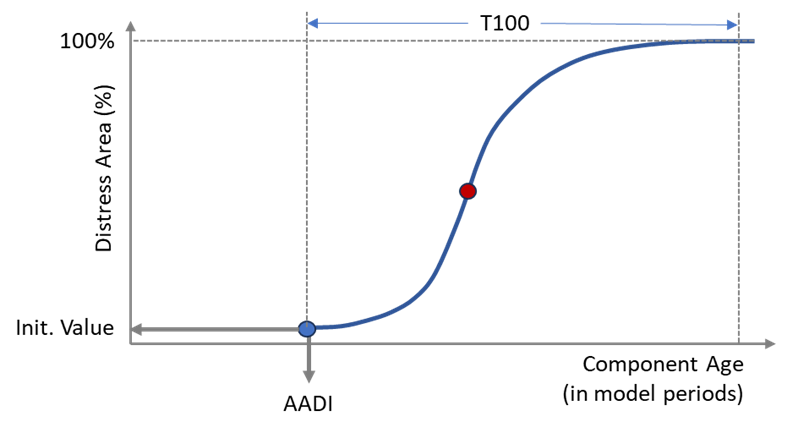
As shown above, this model is characterized by three parameters:
AADI = Age at Distress Initiation.
IV = Initial Value, i.e. percentage distress in the first year when distress initialises.
T100 = Number of years to theoretically reach 100% distress.
Of the above three parameters, AADI is the most important for short to medium term models. In Juno Cassandra, the S-Shape Progression JFunction is used to express these distress parameters. Details on how this model is expressed in Juno Cassandra can be found at this link.
The values for AADI, IV and T100 are not known, and need to be estimated for each segment. In the Default Road Network model, we do this by expressing these values as functions of:
the Expected Surfacing life; and
the Probability of Observing Distress.
The way in which these two elements are used to estimate AADI, IV and T100 are described below.
Expected Surfacing Life
This is a value, expressed in years, that is estimated in two ways: (a) using the estimated surface life for each surface material type value held in RAMM (and downloaded with the input set from JunoViewer); and (b) through analysis and client liaison before the modelling process starts.
Method (a) – i.e. RAMM expected life values - is used during the model initialisation process while method (b) expected life based on historic data analysis and client liaison - is used to reset expected life when a treatment is applied. The reason for using method (a) in the initialisation process is to ensure a smooth transition from the Remaining Surface Life values held in RAMM/Juno and the modelled values after treatment, thereby ensuring better congruency between model outputs and currently held values.
In Cassandra, the expected life using method (b) is expressed in a lookup table such that the expected surface life after treatment can be determined based on:
Surface Material Type (e.g. ‘CHIP2’, ‘RACK’, ‘SMA’).
Urban/Rural Situation.
Pavement Use code.
Thus, when a new treatment is applied, the expected life is looked up based on the above three variables. Before modelling starts the modeller should ideally analyse historic surfacing data to obtain mean achieved surface lives for each unique combination of material type, urban/rural situation and pavement use code. The historically achieved lives should be discussed with the client and finalised in the model lookup tables before the model run starts.
Because expected life is used in the estimation of AADI, IV and T100, and by incorporating client knowledge of the network with historically achieved surface lives, the distress models are implicitly calibrated for the network in question. This is because, in the model, whenever a surface gets older than the expected surface life, the distress will start to initialise. Since the expected surface life is based on historically observed values coupled with client knowledge, calibration is implicitly achieved.
Probability of Observing Distress
For each distress, a Logistic Regression model was fitted on historical data gathered on several New Zealand Local Authorities. These models provide an estimate of the probability of observing the distress in different situations. Here, by ‘situation’ we mean the variables that define a specific road situation, such as:
Traffic (ADT and Heavy Vehicles)
Urban/Rural Situation
Pavement and Surfacing Age
Surfacing thickness and number of layers
Percentage of other distresses that influence the distress in question.
The combination of surface expected life and probability of observing distress facilitates the estimation of AADI. The following method was adopted for the NZLA models:
Table 1: Models for Estimating S-Curve Parameters based on Road Situation
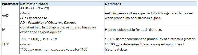
The estimated distress probability provides a way to take account of the situational factors (such as traffic, pavement age etc.) that are likely to influence the time to distress initiation as well as the rate of distress progression. Thus, the estimated distress probability, coupled with the Expected Surfacing life, are the key determinants that express how fast distress will initialise and progress on each element based on the unique situation of the element, coupled with the surface type.