Validation Workflow
Overview
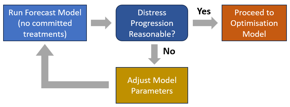
Once your model is up and running, the first step is to assess/validate the reasonableness of your model’s predicted deterioration rates. This process is shown below, and involves running your model in Forecast Mode without providing any committed treatments.
You should prepare for this process by analysing historic network performance under the historic maintenance funding regime. At the least, you should have answers to questions such as:
Did the network aggressively deteriorate over the past 10 years?
Is Rut depth a problem (on many Local Authority networks rutting is quite stable)
Are potholes, cracking etc rapidly changing or staying relatively stable?
Since a Forecast Model does not trigger any new treatments, and since you are also not providing any committed treatments, your outputs will reflect the deterioration of the network in the abscence of any maintenance or renewals. We recommend that you use a forecast period of 15 to 20 years and define a KPI setup that will give you mean values for key condition parameters, such as:
Flushing percentage (‘para_flush_pct’)
Scabbing percentage (‘para_scabb_pct’)
L&T Cracking percentage (‘para_lt_cracks_pct’)
Mesh Cracking percentage (‘para_mesh_cracks_pct’)
Shoving percentage (‘para_shove_pct’)
Pothole percentage (‘para_poth_pct’)
Rut depth (‘para_rut’)
Roughness (‘para_naasra’)
After performing your Forecast Run, use Cassandra’s Post-Processing tool to view a KPI Set over the modelling period.
What To Look Out For
Unless the network has been rapidly deteriorating over the past 10 years, your KPI analysis should show distresses that slowly ramp up from the current baseline, perhaps increasing by 20% to 50% over a 10 year period. After 10 years of no maintenance, it is reasonable to expect that deterioration will accellarate.
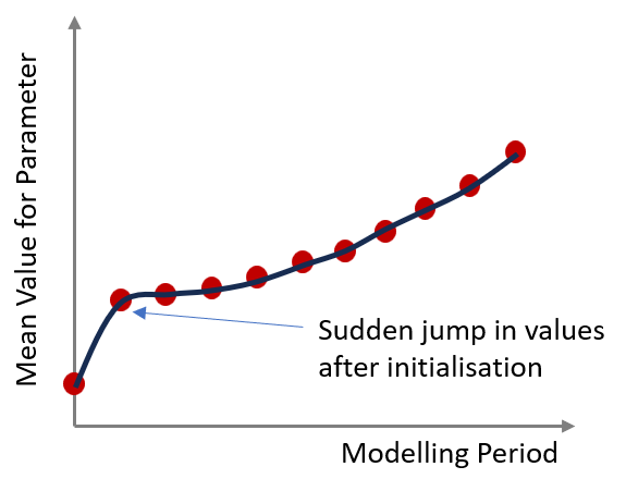
You should not see sudden jumps in deterioration. For example, if your predicted deteriration for a distress starts at a value of 4.0, then jumps to 8.0 and after that stabilises to 8.2, 8.5 etc., then that is often an indication of problems with the calibration based on historic trends, or some sort of threshold being exceeded somewhere. Figure 2 illustrates this situation:
What To Change
Rut Depth and Naasra
If Rut or Naasra is deteriorating too aggressively or too slowly, you can consider changing the central tendency of the increment distribution. At present (November 2025) this can only be done by modifying the C# model code. However, a new release of the model in early December will allow you to configure these parameters in the Lookup tables.
If the calibrated initial rut or roughness rates seem too high or low, you can also adjust the ‘settling-in’ values that are used to estimate the historic deterioration rates. Reducing the setting in values will increase the estimated deterioration rate because less rut or roughness is attributed to ‘settling-in’ and more to deterioration.
Visual Distressses
As explained on this page, distress probabilities are used to determine the AADI relative to the Surface Expected life. One of the key factors that play a role in estimating the probability of distress on a specific segment, is the Pavement Risk factor based on traffic loading and pavement life achieved (model parameter: ‘para_hcv_risk’).
The Pavement Risk Factor is dependent on the Heavy Vehicle Volume and the Pavement Life Achieved. Since the latter is in turn dependent on the Pavement Age and Pavement Expected life, you can increase or decrease the rate of deterioration by adjusting the expected pavement lives used by your model.
If you want to explore this option, you should first adjust the values in your input set (column: ‘file_pave_remlife’). Secondly, you can modify the values in the lookup set that assigns expected pavement life after treatment.
For visual distresses that deteriorate too fast or too slow, you can modify the thresholds for the S-curve parameters such as the minimum and maximum allowed for AADI and T100. See this section for details on adjusting these parameters. Adjusting the minimum or maximum thresholds to T100 is perhaps the best starting place.
Currently, apart from potholes, you cannot adjust the S-curve parameters for distresses individually. That is, the AADI, T100 and Initial value thresholds apply to either potholes or to all other distresses. This simplification is simply to reduce model complexity and prevent the number of calibration parameters from getting out of hand. This is something we plan to address in future improvements of the model.
Since AADI and T100 are dependent on the Expected Surfacing Life, you can also consider adjusting the Expected Surfacing Life values for different surface classes. Reducing surface lives will make the model slightly more aggressive, and increasing surface lives will make the model slightly less aggressive.
If you want to explore this option, you should first adjust the values in your input set (column: ‘file_surf_life_expected’). Secondly, you can modify the values in the lookup set that assigns expected surface life AFTER treatment.
PDI and SDI
Since PDI and SDI are dependent on visual distresses, changes made as suggested above will also influence PDI and SDI.
One additional factor that influences PDI is the weight given to potholes, which we termed the pothole boosting factor. If your PDI seems to deteriorate too aggressively, this can be due to a too aggressive pothole deterioration coupled with an undue influence of potholes on the PDI. You can control the influence of potholes on the PDI by increasing or decreasing the pothole boosting factor.
Surface Remaining Life
Surface Remaining life is basically a ‘bookkeeping value’ since it is directly dependent on surface age relative to the Expected Surface life. You can change the expected surface lives used by your model, it will not affect the rate at which your remaining surface lives change. However, it will affect the starting values and breakdown of remaining surface life.
If you want to explore this option, you should first adjust the values in your input set (column: ‘file_surf_life_expected’). Secondly, you can modify the values in the lookup set that assigns expected surface life AFTER treatment.
When you are calibrating or adjusting your model based on a Forecast Run without treatments, always take into account that your model is not applying any RESET values. This means that the model relies significantly on values in your INPUT DATA - specifically expected surfacing lifes and pavement remaining lives - since the values for these parameters in the lookup sets only come into play after a treatment is applied.