Domain Model Setup

Overview

To define a new Domain Model you need to first get a Model Setup Definition Template file. This template will contain all of the sheets, with their required headers. You can then start building your model using this template as a basis.

In reality, you will almost always start from an existing model template, and then modify that template as needed. If you are uncertain where to start, we recommend that you contact Lonrix for support. We can provide you with the necessary templates and with advice on how to build the model you need.

Once you have created your domain model, you need to provide configuration data to define the model. The required data consist of various sets of tabular data, each set containing key information that informs Juno Cassandra of the following elements:

Model Decision Logic contained in JFunction declarative syntax
The structure of your Input Data file - specifically the headers/columns in your input data file.
Model parameters - the names and properties of the parameters you want to model.
Treatments - the names, categories, unit rates etc. of the Treatments you want to include in your model.
BCA Strategies - the candidate treatment strategies to consider for Benefit-Cost Analysis optimisation.
MCDA Treatments - the candidate treatments to consider for Multi-Criteria Decision Analysis optimisation
MCDA Optimisation Setup - the setup for MOORA ranking if you are using Multi-Criteria Decision Analysis to select optimal strategies.
Lookup tables you want to use in your model.

Important

For Cassandra Desktop, your model is defined in a Domain Model Setup file, which is an Excel file with a specific format. You point Cassandra to this file location when you define your Work Bench.

Cassandra will automatically read your Domain Model setup from this file before each model run starts. You can leave the Model Setup file open while you use Cassandra, but make sure that you save each time after making changes and before you start a new model run.

Each of the above aspects of your Model Input data is described in detail in the sections that follow.

JFunction Set

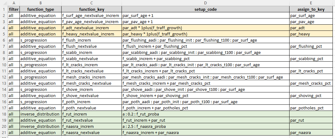
You need define your set of JFunctions in your model definition file on a sheet named ‘function_set’. More details about the structure of your JFunction set can be found in this section. The figure below shows an example of a JFunction set.

In the model input file for the desktop version, the JFunction definition table is expected to be on the mandatory sheet named ‘function_set’.

Input Data Headers

The table for definition of input data headers contains the following columns:

‘column_name’ : name of the column in your input data.
‘data_type’ : data type for this column in your input data. Valid values are ‘number’ or ‘text’.

An example of the raw headers table in the desktop version input file is shown below. In the model input file for the desktop version, the input data header definition table is expected to be on the mandatory sheet named ‘input_headers’.

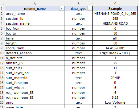
As shown in the figure above, in the desktop version’s input sheet you can add additional columns such as the ‘Example’ column shown above. However, you must have the two mandatory columns in this setup table.

The purpose of the input data headers table is to inform Cassandra of the expected data structure in your input data. Specifically, this set tells Cassandra what column names are to be expected, and the data type. Since your input data is a text file, data in columns with data type ‘numeric’ will be converted to numbers at the start of the model run.

Important

Cassandra will do a check at run time to ensure your input data conform to the definition provided in this setup table. If you input data has fewer columns that what is specified here, you will be informed about this and then the model run will be stopped. You should fix such discrepancies by either modifying your input data, or by modifying this setup table.

Model Parameters

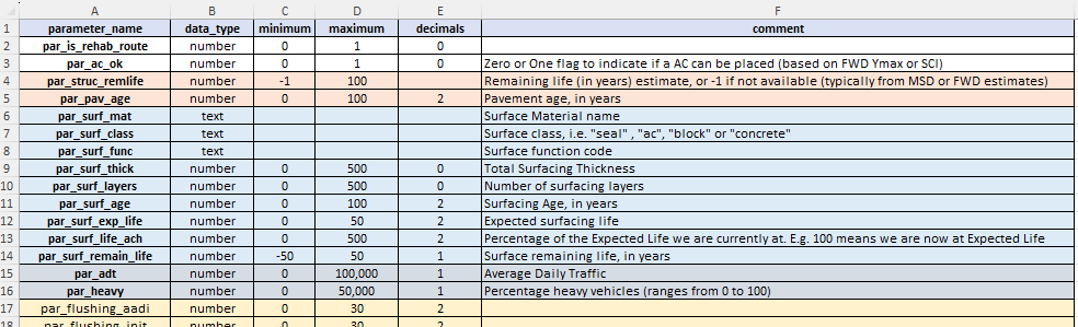
The model parameters setup table needs the following columns:

‘parameter_name’: containing the name of the model parameter. Model parameter names must be prefixed with ‘par_’ or ‘param_’ and must be single words without any special characters (except underscores).
‘data_type’: specifying the type of data for the parameter. Valid values are ‘number’ and ‘text’ (assume case sensitive).
‘minimum’: the minimum allowed value (for numeric parameters only)
‘maximum’: the maximum allowed value (for numeric parameters only)
‘decimals’: the number of decimals to round data to when exporting or displaying data in tables.
‘comment’: a column where you can put optional comments to explain the purpose of each parameter. The column is mandatory, but you can leave some or all values empty if you prefer.

An example of the Model Parameter definitions table in the desktop version input file is shown below. In the model input file for the desktop version, the Model Parameters table is expected to be on the mandatory sheet named ‘parameters’.

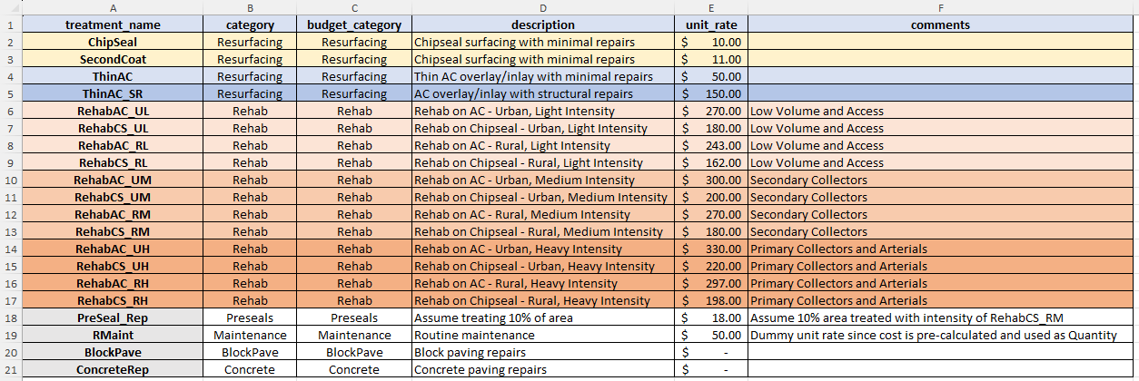
Treatments Definitions

The treatments you want to consider in your model are defined in a Treatments Definitions table. This table requires the following columns:

‘treatment_name’: name for the treatment. This should be a short code without any spaces or special characters.
‘category’: treatment category for grouping treatments for reporting purposes. This should be a single word without special characters.
‘budget_category’ : budget category in which this treatment resorts. The budget category can be the same as the ‘category’ or it can be a different name. For example, if you want to use a monolithic budget (as opposed to a categorised budget), you can set the budget category for all treatments to a single value such as ‘mono’.
’ description’: a short treatment description.
‘unit_rate’: unit rate for the treatment (See note on Unit Rate below).
‘comments’: any comments you want to add for each treatment. The column is mandatory but you can leave the values empty if you wish.

An example of the Model Parameter definitions table in the desktop version input file is shown below. In the model input file for the desktop version, the Treatment Definitions table is expected to be on the mandatory sheet named ‘treatments’.

Note on Unit Rate: The unit rate that you specify for each treatment will be multiplied with the quantity that is calculated at runtime for each strategy. It is up to you to ensure that the Unit Rate is congruent with the Quantity that is set at run time for each treatment. See the ‘Strategy Setup’ below for more information.

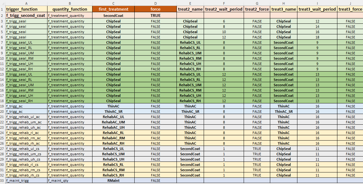
Benefit-Cost Analysis - Strategies Definitions

The strategy definitions table defines all of the treatment strategies that you want to consider as candidates in the Benefit-Cost Analysis (BCA) optimisation approach. In this context, a ‘strategy’ comprises or a sequence of treatment spaced a specified number of years apart. You can create as many strategies as you want in this table. Each strategy - if triggered - will be evaluated over the look-ahead period to determine Life-Cycle Costs and Benefits (relative to a Maintenance-Only scenario).

The following columns are needed in the Strategy Definition Table:

‘trigger_function’: key that identifies the JFunction equality that determined whether this strategy can be considered as a candidate for the current element and its condition.
‘quantity_function’: key that identifies the JFunction that specifies or calculates the effective quantity to be treated. This quantity can map to a constant value (e.g. the ‘area_m2’) column in your input data, or it can be an equation that calculates the effective treatment area as a function of condition etc. Treatment cost will then be determined using this quantity multiplied by the unit rate for the Treatment Type, and discounted to the base year.
‘first_treatment’: name of the first treatment in the strategy. This should be one of the treatment names in the Treatment Definition table.
‘force’: A ‘TRUE’ or ‘FALSE’ flag to indicate whether or not the strategy should be forced. If a strategy that is marked as ‘forced’ is triggered, it will not be evaluated in optimisation but will be forced into the programme before optimisation of other candidate strategies start.
‘treat2_name’: Name of the second treatment in the strategy. Leave empty if there is no second treatment in the strategy.
‘treat2_wait_period’: Number of periods after the first treatment to wait before the second treatment is considered. Leave empty if there is no second treatment in the strategy.
‘treat2_force’: A ‘TRUE’ or ‘FALSE’ flag to denote whether the second treatment should be forced into the programme with the first treatment. See note below. Leave empty if there is no second treatment in the strategy.
‘treat3_name’: Name of the third treatment in the strategy. Leave empty if there is no third treatment in the strategy.
‘treat3_wait_period’: Number of periods after the second treatment to wait before the third treatment is considered. Leave empty if there is no third treatment in the strategy.
‘treat3_force’: A ‘TRUE’ or ‘FALSE’ flag to denote whether the third treatment should be forced into the programme with the first treatment. See note below. Leave empty if there is no third treatment in the strategy.
‘treat4_name’: Name of the third treatment in the strategy. Leave empty if there is no fourth treatment in the strategy.
‘treat4_wait_period’: Number of periods after the second treatment to wait before the third treatment is considered. Leave empty if there is no fourth treatment in the strategy.
‘treat4_force’: A ‘TRUE’ or ‘FALSE’ flag to denote whether the third treatment should be forced into the programme with the first treatment. See note below. Leave empty if there is no fourth treatment in the strategy.
‘reason_function’: Key to the JFunction that determines the Comment to place next to the first treatment if this strategy is selected. This JFunction will typically be a Concatenate Function of several other JFunction keys or parameter values.
‘comment_function’: similar to the ‘reason_function’ above, this should be the key for the JFunction that determines the Reason to place next to the first treatment if this strategy is selected. This JFunction will typically be a Concatenate Function of several other JFunction keys or parameter values.

An example of the Treatment Strategy definitions table in the desktop version input file is shown below (showing only some columns because of space limitations). In the model input file for the desktop version, the Strategy Definitions table is expected to be on the mandatory sheet named ‘bca_strategies’.

Note

In the Juno Cassandra framework, a treatment strategy is a way to evaluate the economic or engineering benefit of a planned sequence of treatments so that this benefit can be compared with a Maintenance-Only option and thereby enable the calculation of costs and benefits to use for optimising available funds using Life Cycle Costs.

It should be noted, however, that when a certain candidate strategy ‘wins’ and is selected for placement, only the FIRST treatment is normally placed into the programme. Follow up treatments will only be placed into the programme if they are marked as ‘forced’.

The reason for this approach is that, when the benefits and costs of a treatment strategy is evaluated, this is done in isolation to the needs and effects on the rest of the network. Since the network needs will change into the future, it does not make sense, while the model is in say period 2, to force a follow up treatment into the programme at period 15.

A more sound approach would be to first roll out the model prediction to period 15 and then evaluate - based on the condition of the network at that stage - how urgent and viable the follow up treatment (which will then be a ‘first treatment’) is in period 15. This is the default process for Juno Cassandra. However, you can override this approach by ‘forcing’ follow up treatments using the appropriate columns as explained above.

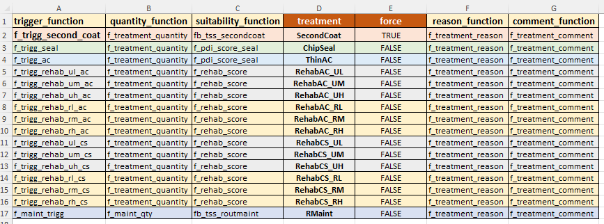
MCDA-Candidate Treatments

This table contains the information needed to set up candidate treatments for use in a Multi-Criteria Decision Analysis (MCDA) type of model. Here, instead of defining a full strategy over the look-ahead period, you only need to define the candidate treatments to consider in an MCDA analysis. Required setup columns/properties are:

‘trigger_function’: key that identifies the JFunction equality that determined whether this treatment can be considered as a candidate for the current element and its condition.
‘quantity_function’: key that identifies the JFunction that specifies or calculates the effective quantity to be treated. This quantity can map to a constant value (e.g. the ‘area_m2’) column in your input data, or it can be an equation that calculates the effective treatment area as a function of condition etc. Treatment cost will then be determined using this quantity multiplied by the unit rate for the Treatment Type, and discounted to the base year.
‘suitability_function’ a key that identifies the JFunction that calculates the relative suitability for this treatment based on the current element condition and other element properties. The suitability score can then be used as one of the factors in your MCDA decision analysis. See this section for details on the Weights and Parameters to use in an MCDA model type.
‘treatment’: Name of the treatment. This name should match one of the names of the treatments defined in the Treatment Definitions table.
‘force’: A ‘TRUE’ or ‘FALSE’ flag to indicate whether or not the treatment should be forced. If a treatment that is marked as ‘force’ = true is triggered, it will not be evaluated in MCDA optimisation but will be forced into the programme before optimisation of other candidate treatments start.
‘reason_function’: Key to the JFunction that determines the Comment to place next to the first treatment if this strategy is selected. This JFunction will typically be a Concatenate Function of several other JFunction keys or parameter values.
‘comment_function’: similar to the ‘reason_function’ above, this should be the key for the JFunction that determines the Reason to place next to the first treatment if this strategy is selected. This JFunction will typically be a Concatenate Function of several other JFunction keys or parameter values.

An example of the MCDA Treatment definitions table in the desktop version input file is shown below. In the model input file for the desktop version, the MCDA Treatments definitions table is expected to be on the mandatory sheet named ‘mcda_treatments’.

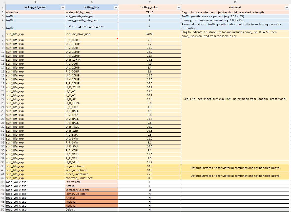
Lookup Table Definition

The lookup table allows you to define any number of ‘lookup sets’, each consisting of a set of key-value pairs. You can use the Lookup JFunction to then look up and extract values from these lookup sets at run time.

Lookup sets typically consist of constants or thresholds that are logically grouped together. For example, you may have one lookup set called ‘surfacing_constants’ which contains thresholds or constants related to surfacing components (for a Road Modelling scenario). Another lookup set may contain ‘trigger_tresholds’ that contain thresholds which play a role in JFunctions that trigger treatment strategies.

The Lookup definition template requires the following columns:

‘lookup_set_name’: A short name for the set. Repeat this name over all rows in the table that belong to this set (see figure below for example).
‘setting_key’: A key for the setting in the lookup set. Setting keys must be unique within a Lookup Set.
‘setting_value’: The value matching the key in ‘setting_key’.
‘comment’: comment to descripe the setting or lookup value.

An example of the Lookup definitions table in the desktop version input file is shown below. In the model input file for the desktop version, the Lookup Definitions table is expected to be on the mandatory sheet named ‘lookups’.

Note

An alternative to using lookup tables is to use separate JFunction Block for each lookup set. Such a JFunction block will typically consist only of Constant JFunctions.

The advantage of such JFunction Blocks instead of a single lookup table set definition is that you can achieve a cleaner separation of elements based on their meaning. With each JFunction block defined in a separate file (desktop version) or table-key (web version), you can more easily manage individual lookup sets.

Multi-Criteria Decision Analysis Setup

The MCDA setup table allows you to define how Multi-Criteria Decision Analysis (MCDA) using MOORA ranking is done if you are using the MCDA model type.

Note that the MCDA Setup is only used when the model type is set to ‘mcda_optimised’. The Treatment Selection mode is defined in the Model Type setting of the Run Configuration

The MCDA setup table requires the following columns:

‘source_type’: Type or source for the ranking parameter. This value should be one of the special/reserved names (see note below).
‘key’: Specific key to define the source for this ranking parameter.
‘weight’: Weight assigned to this ranking parameter in the MOORA ranking process. Cassandra will do a check to ensure that all weights add up to 1.0
‘obj_type’: A 1 or -1 value where: 1 = parameter should be maximised (typically used for positive attributes); and -1 = parameter should be minimised (typically used for negative attributes such as cost).

The following values are allowed for the ‘source_type’ column defined above (case-sensitive):

‘mcda_ranking’ :

Use one of the special parameters extracted from the Treatment Triggering process associated with MCDA analysis. The values you can use for this source type are:

‘treatment_suitability_score’ : Use this code to use the Treatment Suitability score as one of your ranking parameters.
‘treatment_cost’ : Use this code to use the inflated-and-discounted treatment cost as one of your ranking parameters.

‘input_data’ :

This source type indicates that the key you provide maps to one of the columns in your input data. The extracted values for this column will be added as ranking parameters.

‘model_param’ :

This source type indicates that the key you provide maps to one of the Model Parameter names. The extracted values for this Model Parameter will be added as ranking parameters.

An example of the MOORA ranking definitions table in the desktop version input file is shown below. In the model input file for the desktop version, the MOORA ranking definitions table is expected to be on the mandatory sheet named ‘mcda_setup’.

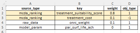
As you can see in the above table, the values in the ‘obj_type’ column are such that Treatment Costs will be minimised (values of -1) while Treatment Suitability Score and ONRC (road hierarchy importance) values will be maximised (values of 1).

Your JFunction that expresses the Treatment Suitability score allows you to assign a suitability score to each treatment. In an MCDA-type model, this treatment suitability score can then be used in conjunction with other criteria (e.g. traffic/volume/cost/importance/risk) in an MCDA analysis to select an optimal set of treatments from amongst the candidates.

Important

Note that the use of a minimum acceptance threshold for the Treatment Suitability Score (assigned in the Run Configuration means that the JFunction expressing your Treatment Suitability Score must always be such that higher scores mean ‘treatment is more suitable’. Because of this, the objective type for the Treatment Suitability Score, as specified for the ‘treatment_suitability_score’ above should always be 1 (indicating maximisation is required). If you do not specify a 1 for the objective type of the ‘treatment_suitability_score’, an error will be thrown at run-time to inform you of this.

Network Functions

JFunctions that are used to calculate initial values, increments and resets are all evaluated at the element level. That is, these functions are calculated on the basis of the values for each element. When calculating these functions, Cassandra does not have any awareness of the overall condition of the rest of the network. This is because - while these element level JFunctions are being executed - the condition of the rest of the network for that epoch is still unknown (because it is in the process of being calculated!).

In some instances, you may want to have access to the condition of the network to make decisions. For example, you may want to calculate - in each epoch - the percentage rank for a certain parameter. To do this, you need to first know all the values for that parameter. Similarly, you want to have a normalised z-score for a parameter. It is the job of Network Functions to facilitate such calculations for you.

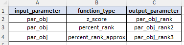
Network functions are defined in a table with the following columns:

‘input_parameter’: this is the name of a numeric model parameter that you want to use for calculating the network-function values. For example, if you want to calculate the percentage rank of a parameter called ‘par_rut’, then you will specificy ‘par_rut’ as the input parameter.
‘function_type’ : this is the type of network-function (see notes below for available types and their codes).
‘output_parameter’ : this is the name of a numeric model parameter that you want assign the calculated network-function values to. For example, if you want to calculate the percentage rank of a parameter called ‘par_rut’ and assign the result to the parameter called ‘par_rut_percent_rank’, then you will specify the output parameter as being ‘par_rut_percent_rank’.

Available Network Function Types:

The following network functions are currently available:

‘z_score’ : use this code for calculating normalised Z-score values.
‘percent_rank’ : use this code for calculating the percentage rank using a highly accurate but slower process. This function will give 100% agreement with the ‘PERCENTRANK()’ function in Excel.
‘percent_rank_approx’ : This method uses Binary Search so it is significantly FASTER than the ‘percent_rank’ method (by a factor of about 100) but when there are many repeat values it does not match the Excel ‘PERCENTRANK()’ function exactly.

Important

It is important to note that Network Functions by necessity need to be calculated after the element level JFunctions have already been evaluated. For example, it is not possible to calculate the percentage rank of a parameter called ‘par_rut’ unless the JFunction that assigns values to ‘par_rut’ has already evaluated for all elements in the network.

Thus, parameter values assigned by Network Functions should always be defined last. That is, they should be the last row or rows in your Parameter Definition Table.

What this constraint means, is that no other parameters can be a function of parameters which are bound to Network Functions. For example, you cannot calculate ‘par_rut_2’ as a function of ‘par_rut_percent_rank’ if ‘par_rut2’ is a JFunction-bound parameter, because JFunction-bound parameters are always evaluated before Network Function bound parameters.

This is a constraint of the current configuration of Juno Cassandra, and future versions may improve this if requested by users. However, users should note that other forms of normalisation such as Min-Max Normalisation can be highly effective and can be implemented using JFunctions.

An example of the Network Function definitions table in the desktop version input file is shown below. In the model input file for the desktop version, the Network Function definitions table is expected to be on the mandatory sheet named ‘network_functions’.

If you choose not to use any Network Functions (the recommended route unless you are a highly experienced modeller), then you can just leave this table blank. That is, leave the table on the specified sheet but without any rows under the headers.