Model Run Configuration
Overview
In the preceding sections, we discussed the key elements that need to be configured before you can run a Cassandra model. After you have defined all the elements that are needed to set up your Project and Domain Model, you should be ready for to start a model run.
The Model Run Configuration is a final set of instructions that instructs Cassandra what options you want to use for a model run. As with Budget Constraint definitions, you can provide a short Name Tag (‘tag’) for a specific model run configuration. When you finally run your model, you can pick which configuration to use for the model run.
Model Run Configurations allow you to specify finer details and options you want to exercise when running a model. This includes aspects that are not defined in either your Domain Model or Project setup data, such as:
- Number of modelling periods to run the model over.
- Type of model to run - see this link for model types.
- Budget Constraint set to use (selected using the Budget Name Tag).
- Whether to trigger Routine Maintenance or not, and whether triggered Routine Maintenance invoke the Reset functions.
- Debug options, such as which elements to export detailed Benefit-Cost data for.
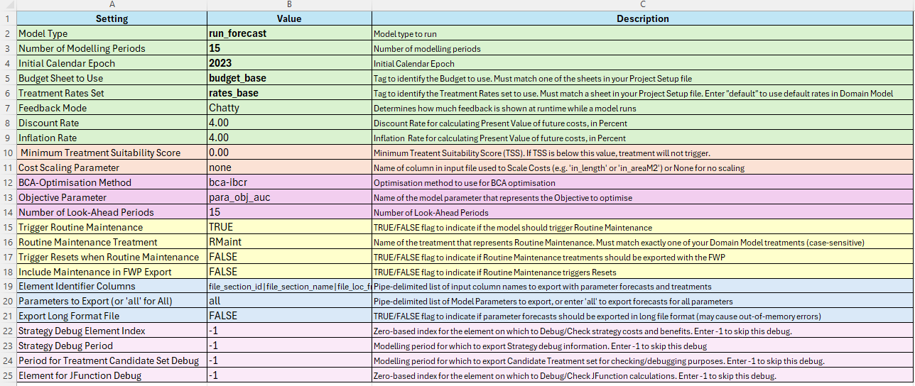
The figure below shows the current table used to define a specific Model Configuration. The sections that follow below provide details on each of the inputs on this form.
Configuration Name Tag
This is the tag you give to your model run configuration. For Cassandra Desktop, you define your Model Configurations in your Work Bench definition file. One worksheet, like the one shown above, can be defined for each configuration.
In the Work Bench file, you define your Model Configurations on sheets starting with the prefix ‘config_’. These sheets will be detected at run-time and you can then choose the configurations to run or view (for post-processing) from the dropbox lists.
Note that when Cassandra reads configurations from your Work Bench set-up file, it will remove the ‘config_’ prefix from your configuration names. Thus, if you define a configuration on a sheet called ‘config_mcda_2023_10_years’, the configuration name tag shown to you in drop down lists will be simply ‘mcda_2023_10_years’.
Run Settings
Model Type Name
This setting specifies the type of model you want to run. The following values for model_type are allowed:
‘run_forecast’ : Cassandra will run a forecast with or without a set of committed treatments. This model does not trigger or assign any treatments. Instead, it tells you what your network’s likely future condition will look like given a certain set of treatments and conditions.
‘bca-optimised’ Cassandra will run a full model with or without committed treatments and with strategy triggering and Benefit-Cost over life-cycle optimisation to suit budget constraints.
‘mcda-optimised’ Cassandra will run a full model with or without committed treatments and with treatment triggering and Multi-Criteria Decision Analysis (MCDA) used to select optimal treatments to suit budget constraints.
Number of Modelling Periods
This is the number of modelling periods over which the model should run. Note that a model period can be a year or month or whatever is defined as a period by your Domain Model.
Typically, where modelling periods represent years, the number of modelling periods will be set to three years for a short-term model, 10 to 15 years for a medium-term model, and 20 to 30 years for a long-term model. Also see this page for a discussion on the difference between a modelling Period and a modelling Epoch.
Initial Calendar Epoch
In Cassandra models, the modelling periods range from one to the number of modelling periods specified in the number of modelling periods setting. For reporting purposes, you will typically want to convert these modelling periods to calendar periods and epochs. The ‘initial_calendar_epoch’ setting allows you to specify the calendar year that corresponds to period zero.
Thus, if your starting date represents the end of 2024, then period 1 will take place between 2024 and 2025, and epoch 2025 will represent the end of period 1. For more details on the concept of epochs and periods, please see this help page.
Budgets Tag to Use
Here you need to specify the name tag of the Budget Constraint set that holds your Budget constraints to use for the model. The drop-down list shown will allow you to pick any Budget Constraint sets defined in your project-level data.
Treatment Rates to Use
Here you need to specify the name tag of the Treatment Rates set that holds your Project-specific Treatment Rates to override in the Domain Model. As with the Budget Tag, the drop-down list shown will allow you to pick any Treatment Rates sets defined in your project-level data..
Feedback Mode
This is the ‘chattiness’ of Cassandra while running models or longer running commands. Options are:
- Chatty : shows all messages including additional debug/feedback and progress messages.
- Somewhat Shy : displays warnings, key messages and progress during execution.
- Introvert : displays only warnings and key progress messages during execution.
- Silent : almost completely silent during execution.
Discount Rate
This is the discount rate, in percent (e.g. a number such as 3.45) to use when discounting future life-cycle costs to present value. Note that, in Cassandra, all costs are converted to Present Value costs before optimisation/exporting/prioritisation. A high discount rate will mean that future costs will be lower than present value costs. If the inflation and discount rates are the same, then discount and inflation rates have no effect on costs.
Inflation Rate
This is the Inflation rate, in percent (e.g. a number such as 3.45) to use when inflating future life-cycle costs from present value costs. Note that, in Cassandra, all costs are converted to Present Value costs before optimisation/exporting/prioritisation. A high inflation rate will mean that future costs will be higher than present value costs. If the inflation and discount rates are the same, then discount and inflation rates have no effect on costs.
Multi-Criteria Decision Analysis (MCDA) Models
Minimum Treatment Suitability Score
This is the minimum Treatment Suitability Score that a triggered treatment must meet in order to be considered a candidate treatment in an MCDA analysis type. The Treatment Suitability score needs to be calculated by your Domain Model using the JFunction specified in the ‘mcda_treatments’ setup table.
Your JFunction that expresses the Treatment Suitability score allows you to assign a suitability score to each treatment. In an MCDA-type model, this treatment suitability score can then be used in conjunction with other criteria (e.g. traffic/volume/cost/importance/risk) in an MCDA analysis to select an optimal set of treatments from amongst the candidates.
Note that the use of a minimum acceptance threshold for the Treatment Suitability Score means that the JFunction expressing your Treatment Suitability Score must always be such that higher scores mean ‘treatment is more suitable’. Because of this, the objective type for the Treatment Suitability Score, as specified in the [in the ‘mcda_treatments’ setup table]domain_model_setup.qmd#mcda-setup-data) should always be 1 (indicating maximisation is required).
More details about the use of the Treatment Suitability score in an MCDA model-type will be provided in later sections of this documentation.
Benefit-Cost Analysis (BCA) Models
Optimisation Method
This code to specifies the optimisation approach to follow when selecting treatments under a budget constraint in a Life-Cycle Cost, Benefit-Cost Analysis (BCA) model. Please specify one of the following options (code is case-sensitive):
- bca-greedy : Benefit-Cost optimisation based on a ‘Greedy’ selection of projects using Incremental Cost-Benefit Ratios (ICBR).
- bca-egal : Benefit-Cost optimisation based on an ‘Egalitarian’ selection of projects using Incremental Cost-Benefit Ratios (ICBR).
- bca-ibcr : Benefit-Cost optimisation based on an ‘Increasing ICBR’ selection of projects using Incremental Cost-Benefit Ratios (ICBR).
Lonrix is working on an additional optimisation method utilising the more rigorous Multiple Knapsack solver using Dynamic Programming. This effort is being supported by Beca Consultants and Lonrix is especially grateful to Lucien Zhang from Beca who provided a foundational algorithm to support these efforts.
More details about each of these above methods will be provided in later sections of this documentation (#TODO). You can also refer to this section to access YouTube videos on the above methods.
Objective Parameter
This is the Name/Code of the modelling parameter that represents to Objective Value from which Benefits will be estimated in Life-Cycle Cost calculations. The value specified here must match one of the model parameter names specified in the Model Setup file.
In Benefit-Cost Analysis (BCA), the objective values are calculated under a given treatment strategy over the specified look-ahead period. The sum of these values represent the ‘area-under-the-curve’ for the objective function. This sum is then subtracted from the same sum as calculated under a ‘Do-Nothing’ (which is actually a ‘Routine-Maintenance-Only’) scenario. The difference between the areas-under-the-curves for the treatment strategy and the Do-Nothing scenario thus represents the ‘Benefit’ that is used in BCA-optimisation.
Number of Look-Ahead Periods
This is the number of periods to consider when evaluating life-cycle costs for Benefit-Cost Analyses. Note that this is not the same as the number of modelling periods. The look-ahead periods determine the duration over which life-cycle costs are evaluated while the number of modelling periods determine how many years into the future the model should run.
It is, for example, possible to run a model over only 10 modelling periods while the look-ahead period is 15 years/periods. This means, in effect, that - for the purposes of evaluating the life-cycle costs of candidate treatment strategies - the model will always run for the number of modelling periods PLUS the look-ahead periods. However, forecast results are output only for the number of modelling periods.
The model run-time is sensitive to the number of look-ahead periods specified. You should make this period only as long as needed to properly evaluate which of the competing treatment strategies offers the best performance over the element’s life cycle. There is little benefit in extending the number of look-ahead periods very far beyond the time of the last treatment in a strategy.
Routine Maintenance
Trigger Routine Maintenance?
Check this box if you want to consider Routine Maintenance in your trigger sequence. If this box is unchecked, routine maintenance will not be triggered.
Routine Maintenance Treatment
This is the name of the treatment type that represents Routine Maintenance. The name you specify here must match exactly (assume case-sensitivity) the name of one of the treatments defined in your model set-up file. If you do not want to trigger maintenance, you can set this value to ‘none’.
Routine Maintenance Triggers Resets
This option determines whether the application of Routine Maintenance should trigger a Reset of condition or not. In many instances, you will want a model that does NOT reset the element condition when routine maintenance is applied, otherwise the Maintenance-Only strategy will tend to always outperform other treatment strategies.
Since Routine Maintenance is generally only a backstop to temporarily address urgent problems, you can bypass the RESET function for routine maintenance by setting the value for this setting to FALSE. In that case, the Increment phase, rather than the Reset phase, will be executed when Routine Maintenance is applied.
Include Routine Maintenance in FWP?
One of the outputs of a model run is a conventional, flat version of the Forward Works Programme (FWP) associated with a model run. Since Routine Maintenance can be triggered much more often than other more periodic treatments, the FWP can be cluttered and hard to analyse if it is largely populated by the Routine Maintenance treatment.
For this reason, this setting allows you to instruct Cassandra to omit the display of Routine Maintenance in the exported FWP. Note that this does not mean that routine maintenance is not applied - it only means that routine maintenance is not shown. Also note that routine maintenance is always included in the Treatments Export file, regardless of whether this setting is TRUE or FALSE.
The Flat FWP output shows treatments in different years in a wide-horizontal format. In this format there is only one row for each element, and different treatments in different periods on the same element are shown in separate COLUMNS.
By contrast, the treatments export file lists treatments in a narrow, long format in which different treatments on the same element appear in subsequent rows. Thus, in the Treatments Export file, there is likely to be more than one row for each element.
Output Settings
Element Identifier Columns
This is a pipe-delimited list of the columns in the Raw Input file that should be included to help identify elements in model export and feedback files. Without these identifier columns, the output will only be listed against the zero-based element index, and users will have to refer back to the raw input file to determine which element is represented by which element index.
The element identifier columns thus provide you with the ability to put fields such as element name, region, etc.
Make sure that the identifier column names you specify match exactly the names of columns in the raw input file. Assume a case-sensitive comparison. If any of the names you specify for this setting are not found in the raw input file columns, a set-up error will be thrown at start-up.
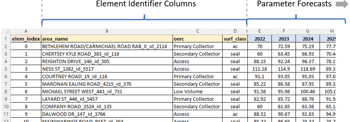
The figure below shows an example of a model output file for a specific model parameter, and shows the element identifier columns directly to the right of the element index column, and to the left of the model parameter forecasted values. To achieve this output, the specified value for the element identifier column setting would have been: ‘area_name|onrc|surf_class’.
Parameters to Export
This is the pipe-delimited list of model parameter names to be exported at the end of the modelling run. OR, you can enter ‘all’ to simply export the data for ALL model parameters. Because the exporting of model data can be time consuming for large numbers of model elements, the use of an explicitly specified list of parameters is useful when you are doing exploratory analysis and only want to check on one or two parameters.
Export Long Format File
If checked, this option will export parameter data in a long, narrow format in which data for all parameters are included in a single output file. Not that this option may lead to a memory overflow in the case where you have a large number of model parameters and elements.
Debug Settings
Element Index for Strategy Debug
This should be the zero-based index (that is, the first element has index zero) of the element for which you want to export details of the Life-Cycle Benefit-Cost data that is generated in a specific year. This can be used to debug or peek into the life-cycle cost information for a specific element in a specific year. Enter -1 if you do not want to apply this for any element.
Strategies Debug Modelling Period
This should be the modelling period at which you want to export the Life-Cycle Benefit-Cost data that is generated for the element specified in the previous setting. This can be used to debug or peek into the life-cycle cost information for a specific element. Enter -1 if you do not want to use this feature in a modelling run.
Debug Treatment Set
This should be the modelling period at which you want to export the full list of treatment strategies with their relative ranking for treatment selection and optimisation. This list can be used to debug which treatments were triggered and what the assigned benefit and cost information associated with each strategy is. Enter -1 to skip this feature in a modelling run.
Element Index for Function Set Debug
This should be the zero-based index (that is, the first element has index zero) of the element for which you want to track and export the full JFunction result set for every period. This is a useful debug feature to track calculations by your JFunctions for a specific element.
All of the files generated for the above-noted debug functions will be written into the ‘debug’ sub-folder of the Work Folder you specify when you set your Work Bench. Note that an error will occur if you open one of these debug output files and keep it open when you start the next model run. So please ensure you always close any open debug or output files before you start a model run.